Forest Cover Type - Kaggle Challenge
Written: August 2018 (Github)
Introduction
Here is a summary of my work on the Forest Cover Type Kaggle challenge. If you would like to see my code, please see my repo on Github.
Background
Kaggle introduces the challenges as follows:
In this competition you are asked to predict the forest cover type (the predominant kind of tree cover) from strictly cartographic variables (as opposed to remotely sensed data). The actual forest cover type for a given 30 x 30 meter cell was determined from US Forest Service (USFS) Region 2 Resource Information System data. Independent variables were then derived from data obtained from the US Geological Survey and USFS. The data is in raw form (not scaled) and contains binary columns of data for qualitative independent variables such as wilderness areas and soil type.
This study area includes four wilderness areas located in the Roosevelt National Forest of northern Colorado. These areas represent forests with minimal human-caused disturbances, so that existing forest cover types are more a result of ecological processes rather than forest management practices.
Variable overview
| Name | Measurement | Description |
|---|---|---|
| Elevation | meters | Elevation in meters |
| Aspect | azimuth | Aspect in degrees azimuth |
| Slope | degrees | Slope in degrees |
| Vertical Distance To Hydrology | meters | Vertical Distance to nearest surface water features |
| Horizontal Distance To Hydrology | meters | Horizontal Distance to nearest surface water features |
| Horizontal Distance To Roadways | meters | Horizontal Distance to nearest roadway |
| Horizontal Distance To Fire Points | meters | Horizontal Distance to nearest wildfire ignition points |
| Hillshade 9am | 0 to 255 index | Hillshade index at 9am, summer solstice |
| Hillshade Noon | 0 to 255 index | Hillshade index at noon, summer soltice |
| Hillshade 3pm | 0 to 255 index | Hillshade index at 3pm, summer solstice |
| Wilderness Area (4 binary columns) | 0 (absence) or 1 (presence) | Wilderness area designation |
| Soil Type (40 binary columns) | 0 (absence) or 1 (presence) | Soil Type designation |
| Cover Type | Classes 1 to 7 | Forest Cover Type designation - Response Variable |
Target: Cover Type
The variable we are trying to predict in the Test data is the variable "cover_type". The cover types are labeled as following:
- Spruce/Fir
- Lodgepole Pine
- Ponderosa Pine
- Cottonwood/Willow
- Aspen
- Douglas-fir
- Krummholz
Furthermore, as we can see below, the cover type is perfectly balanced within the training data
Datasets
As this is a classification challenge, the data is split between train data (data with target) and test data (data without target). As a challenge, the test data is over 35x as big as the train data!
Correlation Plot
Hydrology
As stated before, the hydrology variables indicate the "distance to nearest surface water features". It's a bit difficult to get any information out of this. However it does appear that Krummholtz and Douglas-Fir are the furthest away from water.
The total distance from water, given by [horizontal distance]^2 + [vertical distance]^2 should be added during feature engineering.
Wilderness Area
Hillshade
There seems to be two latent variables that are given by the three hillshade values. The relationship definitely looks 2 dimensional and forms a plane.
Shade, Slope, and Elevation
Elevation seems to be a very important feature to look at when deciding the cover type. In addition, hillshade and slope seem to have a planar boundary that cuts off values.
Soil Type
There 40 different soil types in this dataset labeled numerically as opposed to the actual name. It's hard to get an understanding of this variable without knowing what each number refers to. However we can notice that the train data and test data look very different. This might lead us to believe that the test data is unbalanced with respect to the target variable unlike the train data. This guess will turn out to be correct.
Fire Points and Roadways
Density Plots
Density plots are an excellent resource for viewing how a variable will change for a given cover type
Elevation
Elevation is perhaps the strongest variable. Looking below it does a great job separating the different forest covers.
Positional variables
These variables indicate the position relative to roadways, fire points, and hydrology.
Remaining variables
Finally, here are density plots for the remaining variables.
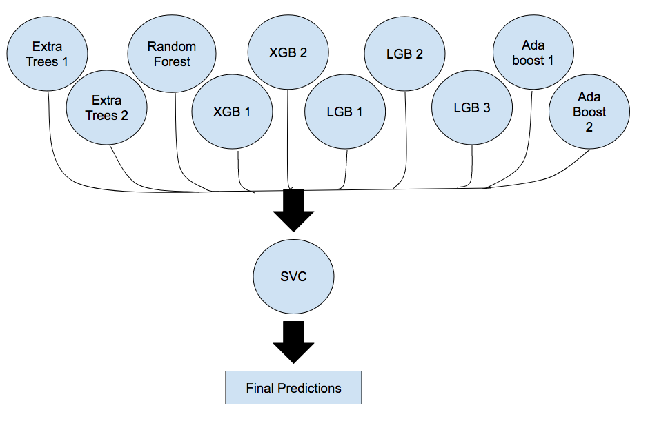
Modeling
An ensemble classifier is constructed to predict the cover types in the test dataset. XGBoost, LGBoost, Ada Boost, Random Forests, and Extra Trees models are trained with predictions stored in a dataframe. These predictions are then fed into a SVC model that gives a final prediction based on the individual predictions of each model. The classifier scores around 81% accuracy on Kaggle's public leaderboard.
Prediction distribution
Interestingly, the predictions are highly inbalanced unlike the training data which is perfectly balanced. The distribution below is not completely correct, but it's good enough with 85% accuracy.
Conclusion
Thank you for viewing this, if you would like to see my code, please see my repo on Github.
Acknowledgements
This dataset is provided by Jock A. Blackard and Colorado State University. A full citation is given below.
Bache, K. & Lichman, M. (2013). UCI Machine Learning Repository. Irvine, CA: University of California, School of Information and Computer Science